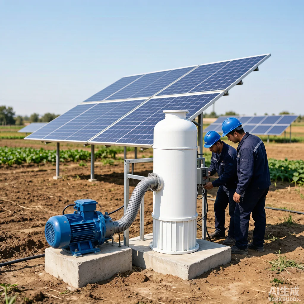
Solar Pump System Design for Variable Water Demand Applications
Introduction
Designing a solar-powered water pumping system becomes significantly more complex when daily and seasonal water demand fluctuates unpredictably. In agricultural cooperatives, rural community water supply networks, and livestock operations, consumption patterns often vary by factors of 3x to 5x between peak and off-peak periods. A rigidly sized system that matches a single design point will either undersupply during critical windows or waste capital on oversized components that idle through most of the year. KINBO, a specialized manufacturer of solar water pumping solutions, approaches variable-demand applications with a layered design methodology that balances solar array capacity, pump staging logic, and hybrid storage architectures. This article explores the engineering principles, quantitative trade-offs, and practical design frameworks that engineers and system integrators can apply when specifying solar pump systems for non-uniform water demand profiles. We examine diurnal, seasonal, and growth-driven variability patterns, compare storage strategies with real cost and efficiency data, outline multi-pump cascade control configurations, and present a decision framework for sizing solar arrays against the peak-versus-average dilemma.
Table of Contents
Understanding Demand Variability Patterns
Variable water demand in solar pumping applications can be decomposed into three superimposed components: diurnal, seasonal, and growth-driven. Each imposes distinct constraints on system architecture, and engineers must model them jointly rather than treating them as independent design cases.
Diurnal variability is the most tractable. In livestock watering operations, cattle typically drink 70–80% of their daily intake between 06:00 and 12:00, with a secondary peak at 16:00–18:00. This intra-day pattern aligns partially with solar irradiance curves — a fortunate coincidence that allows direct-coupled systems to meet morning peak demand when insolation is rising. However, the afternoon gap (13:00–15:00) often sees demand troughs when irradiance peaks, creating surplus energy that must be stored as pumped water or diverted. Community water supply systems exhibit a different diurnal shape: morning cooking/cleaning peaks (06:00–09:00) and evening peaks (17:00–20:00) that bookend the solar window, making storage indispensable.
Seasonal variability introduces far greater design tension. Crop irrigation in temperate zones can swing from near-zero winter demand to 40–60 m³/day per hectare during mid-summer. A system sized for July peak load would operate at 15–25% capacity factor through winter months — economically wasteful and technically problematic since permanent-magnet motors lose efficiency below 30% rated speed. In tropical regions with wet/dry seasons, the inverse problem emerges: peak water demand during the dry season coincides with peak solar resource, but the system must still handle transitional-month variability.
Growth-driven variability is a planning consideration rather than an operational one. Agricultural enterprises, community water schemes, and livestock operations rarely maintain static demand over a 10-year horizon. A modular design philosophy — where pump bays, racking structures, and controller capacity accommodate future expansion without upfront oversizing — delivers the lowest lifecycle cost. KINBO’s system design methodology recommends specifying controllers with 30–40% I/O headroom and sizing cable conduits for one gauge heavier than immediate load requires, adding negligible first cost (typically 3–5% of total project cost) while enabling cost-effective capacity upgrades.
Hybrid Storage Solutions: Elevated Tanks vs Ground Reservoirs vs Pressure Tanks
Storage strategy is the single most consequential design decision in variable-demand solar pumping. The three primary options — elevated tanks, ground-level reservoirs, and pressure vessels — differ substantially in capital cost, energy efficiency, water quality implications, and operational complexity.
Elevated storage tanks provide gravity-fed distribution pressure (0.43 psi per foot of elevation, or approximately 1 bar per 10 meters of head), eliminating the need for secondary booster pumping. A 10,000-liter tank elevated to 15 meters delivers roughly 1.5 bar at the distribution point — adequate for drip irrigation laterals and low-rise community standpipes. The capital cost premium is significant: reinforced concrete tower structures add $12,000–$18,000 to a 10 m³ system in most developing markets, and steel panel tanks on welded towers run $8,000–$14,000. However, the elimination of distribution pumping energy (typically 0.3–0.6 kWh/m³ for horizontal distribution) yields a 5–8 year payback on the tower investment in systems pumping more than 20 m³/day.
Ground-level reservoirs (lined ponds, concrete basins, or sectional steel tanks) minimize civil works cost at $3–$8/m³ of storage, but require secondary pressurization for distribution. A 50 m³ lined pond costs roughly $2,500–$4,000 in materials and excavation, versus $45,000+ for equivalent elevated storage. The trade-off is ongoing energy expenditure: a 1.5 kW booster pump consuming 4–6 kWh/day adds approximately $400–$600/year in electricity costs (at $0.10–$0.15/kWh) or requires additional solar capacity of 1.2–1.8 kWp at roughly $800–$1,200 incremental array cost.
Pressure tanks (bladder or diaphragm type) serve a fundamentally different function: they buffer short-duration flow transients and reduce pump cycling frequency rather than storing bulk water volume. A 200-liter pressure vessel with a 40/60 psi cut-in/cut-out range stores approximately 50–60 liters of usable water between cycles — enough to serve intermittent domestic demand without triggering pump starts for every tap opening. In solar pumping, pressure tanks reduce motor inrush current events that stress inverter components. KINBO recommends pressure tank sizing at 10–15 liters per 100 W of pump motor rating for household-scale systems, and combined ground-reservoir-plus-pressure-tank architectures for community systems over 5,000 L/day.
Hybrid configurations — a ground reservoir for bulk solar-hour storage with a smaller elevated tank or pressure vessel for distribution — consistently achieve the best capital-to-operational cost ratio. A representative 20 m³/day community system in Sub-Saharan Africa using a 30 m³ lined reservoir, 1.5 kW submersible solar pump, and 5 m³ elevated header tank with float-switch control reports total installed cost of $11,500–$14,000 and 92–94% water delivery reliability across seasonal demand swings.
Multi-Pump Staging and Cascade Control Design
When demand variability exceeds a 3:1 ratio, a single pump operating across its full speed range cannot maintain acceptable efficiency. Permanent-magnet synchronous motors (PMSM) in solar submersible pumps achieve 85–92% peak efficiency at 70–100% of rated speed, but efficiency collapses to 50–65% below 30% speed due to fixed excitation losses and bearing friction. Multi-pump staging — deploying two or more pumps of different capacities or identical pumps in parallel — confines each unit to its high-efficiency operating band and improves overall wire-to-water efficiency by 12–18 percentage points in variable-demand applications.
Cascade control logic governs which pumps run and at what speed based on system pressure, flow demand, or storage tank level. A typical three-pump cascade (small/medium/large or 2+1 parallel configuration) uses the following staging rules:
| Demand Range (m³/h) | Active Pumps | Operating Mode | System Efficiency |
|---|---|---|---|
| 0–1.5 | Pump 1 (2 HP) | VFD 30–100% speed | 72–88% |
| 1.5–3.5 | Pump 2 (5 HP) | VFD 40–100% speed | 78–91% |
| 3.5–6.0 | Pump 1 + Pump 2 | Parallel, speed-matched | 80–90% |
| 6.0–9.0 | Pump 3 (10 HP) | VFD 50–100% speed | 82–92% |
| 9.0–15.0 | All three pumps | Parallel, speed-matched | 78–88% |
The controller monitors a combination of pressure transducer feedback (for closed-distribution systems) and ultrasonic tank level sensors (for storage-fill applications). Staging transitions incorporate a 30–60 second hysteresis delay to prevent oscillation between stages — a common failure mode in poorly tuned cascade systems that causes excessive contactor cycling and premature pump wear.
For larger installations (above 15 m³/h peak demand), KINBO recommends a master-slave architecture where a central PLC or smart pump controller manages up to six pump drives via Modbus RTU communication. Each pump’s VFD reports real-time power draw, speed, and estimated flow (derived from the pump’s factory-characterized power-to-flow curve), enabling the master controller to optimize the pump combination for highest wire-to-water efficiency rather than simple sequential staging. Field data from a six-pump irrigation installation in Kenya shows 23% lower daily energy consumption compared to fixed sequential staging at the same total daily flow volume.
Sizing Solar Arrays for Peak vs Average Demand Trade-offs
The fundamental tension in sizing the photovoltaic array for variable-demand systems is between two competing objectives: meeting peak-day demand (typically 95th–99th percentile) versus minimizing the levelized cost of water (LCOW). An array sized for the 99th percentile demand day will satisfy nearly all demand but operate at low capacity factor through most of the year, inflating capital cost per cubic meter delivered. An array sized for average demand leaves a deficit on peak days that must be covered by storage or supplemental energy.
The economic optimum emerges from the interaction of three parameters: array cost ($/Wp installed), storage cost ($/m³), and the demand coefficient of variation (CV = standard deviation / mean). As a practical design rule derived from KINBO’s project database across 40+ installations in Africa and Southeast Asia: when the monthly demand CV exceeds 0.35, supplementary storage is almost always cheaper than incremental array capacity for meeting peak-day requirement. When CV is below 0.25, oversizing the array by 15–25% beyond average-day requirement is typically the lower-cost path.
A worked example illustrates the framework. Consider a livestock operation with the following monthly demand profile:
- Average daily demand: 15 m³/day
- Peak month (July) average: 28 m³/day
- Peak day within peak month: 35 m³/day
- Solar resource: 5.5 PSH (peak sun hours) annual average, 6.2 PSH in July
- Total dynamic head: 45 meters
Array sizing for average demand: Hydraulic energy required = 15 m³ × 45 m × 9.81 / 3,600 = 1.84 kWh/day hydraulic. With 55% wire-to-water system efficiency and 5.5 PSH, required array = 1.84 / (0.55 × 5.5) = 0.61 kWp. With 1.2x derating for temperature and soiling, installed capacity ≈ 0.73 kWp (roughly three 250 W panels).
Array sizing for peak day: 35 m³ × 45 m × 9.81 / 3,600 = 4.29 kWh/day hydraulic. Required array = 4.29 / (0.55 × 6.2) = 1.26 kWp. With derating, ±1.51 kWp (six 250 W panels).
The incremental cost of six panels versus three panels (400 W panels at $0.35/W installed) is roughly $420. The incremental storage cost for bridging 20 m³ of peak-day deficit (35–15 m³) is a 30 m³ lined reservoir at approximately $1,800–$2,400 or a 20 m³ sectional steel tank at $3,000–$4,000. In this case, the modest array oversizing (plus a smaller 10 m³ buffer tank at ±$1,200) delivers the optimal lifecycle cost: roughly $1,620 total incremental investment versus $1,800+ for storage-only solutions, and with zero recurring pumping energy penalty. KINBO’s design tools automate this multi-variable optimization for site-specific load profiles and equipment cost data.
Frequently Asked Questions
Q: How do you size a system when demand varies 5x between seasons?
A: A 5:1 seasonal swing is severe enough that neither array oversizing nor storage alone provides an economical solution. The recommended approach is a two-stage design: size the solar array for 110–120% of the average seasonal demand (not peak), then deploy sufficient water storage to bridge the peak-season deficit using solar energy accumulated during off-peak periods. For a system averaging 10 m³/day but peaking at 50 m³/day for two months, the array is sized for 11–12 m³/day average output. During the two peak months, the 38 m³/day deficit (50 – 12 = 38 m³/day) multiplied by 60 days equals 2,280 m³ of total storage requirement. In practice, a 2,500 m³ lined reservoir or pond is constructed. Off-peak solar energy fills it gradually; peak-season demand draws it down. This approach typically saves 40–55% on array capital cost compared to peak-sizing, with storage cost of $3–$6/m³ for lined earthworks in most markets. A VFD-controlled pump set with two or three parallel units maintains efficiency across the wide flow range. KINBO engineering teams can model this trade-off for specific site coordinates and load data.
Q: Is battery storage better than water storage for solar pumps?
A: For the vast majority of solar pumping applications, water storage is economically and technically superior to battery storage, by a substantial margin. The cost comparison is decisive: storing 1 kWh of potential energy as pumped water in an elevated tank costs approximately $0.02–$0.15/kWh of storage capacity (amortized over the tank’s 20–25 year service life), while lithium-iron-phosphate (LFP) battery storage costs $0.12–$0.25/kWh per cycle at current prices — roughly two orders of magnitude more expensive per unit of delivered energy over the system lifetime. Water tanks have 20+ year lifespans with negligible degradation; batteries degrade to 70–80% capacity within 8–12 years and require climate-controlled enclosures. There are specific exceptions where batteries may be justified: (1) ultra-deep wells (>300 m head) where elevating water for storage imposes excessive pumping energy losses, (2) sites with severe land constraints that preclude reservoir construction, and (3) applications requiring precise pressure control where a small battery bank (2–5 kWh) stabilizes DC bus voltage for the pump inverter. In these edge cases, KINBO specifies hybrid systems with minimal battery capacity — typically 3–6 kWh LFP — sufficient only to buffer solar variability and avoid pump cycling, not for bulk energy shifting.
Q: What is the minimum flow rate for intermittent demand?
A: The minimum sustainable flow rate for intermittent-demand solar pumping is determined not by the pump’s physical minimum (most solar submersibles can operate stably down to 10–15% of rated flow) but by two practical constraints: motor cooling and inverter minimum power point tracking (MPPT) window. Submersible motors rely on water flow past the motor housing for convective cooling. Below approximately 0.15–0.2 m/s flow velocity across the motor surface, internal winding temperatures rise above the Class F insulation rating (155°C), accelerating insulation degradation. For a typical 4-inch submersible in a 6-inch casing, this translates to a minimum flow rate of roughly 1.2–1.8 m³/h, depending on ambient water temperature. The inverter MPPT constraint arises because at very low irradiance (below 150–200 W/m²), the DC bus voltage may fall below the pump inverter’s minimum input threshold, causing repeated start/stop cycling rather than continuous low-flow operation. For intermittent demand applications, KINBO recommends configuring the controller with a “minimum runtime” setting of 3–5 minutes once started, combined with a pressure tank or small elevated header tank (100–500 liters) to buffer demand during low-irradiance periods. This configuration supports reliable intermittent flows as low as 0.5 m³/h on a 1.5 kW system without excessive cycling.
Need expert guidance on designing a solar pump system for your variable-demand application? Contact the engineering team at KINBO for site-specific system sizing and a detailed techno-economic analysis.